Quantum Mechanics Simulations

[Posted here for login-free access from public computers.]

Note: For the “lab report,” answer all questions marked as Q1, Q2, etc. on separate pieces of paper to turn in. Use the space provided in the lab manual for graphs or answers required to be formatted in a particular way. Please follow all directions and answer all questions. You only need to turn in your answers for the lab report. Write your name and your group partners’ names on your lab report.

Introduction

By now, we have been discussing experimental results that led to the development of quantum mechanics, some of the key assumptions (initially ad hoc, later more formalized) that form the starting points for quantum mechanics. There are two main difficulties in correctly understanding quantum mechanics beyond simply memorizing some formulas, like the energy levels in the Bohr model: (1) No one comes in with any level of intuitive understanding for quantum mechanics. Your intuition is based on situations you have encountered and have some experience with. Because the quantum mechanical effects most clearly become manifest in microscopic (or even subatomic) situations, your everyday experience did not help you develop any intuition for quantum mechanics. (2) The mathematics of quantum mechanics is challenging, involving fair amount of calculus, and at times, linear algebra (the kind with complex linear vector space).

Our goal in this lab is to help you develop some intuition for the wave mechanics formulation of quantum mechanics, exploring the consequences of the de Broglie hypothesis, that everything that has a momentum has a wavelength, and that they are related by the expression, $LaTeX: p=h/\lambda$ . We will use numerical computer simulations to help bypass the issue (2) for now. (I believe it’s the job of your upper-division quantum-mechanics class to teach you how to actually handle the math involved.)

Part A: Wave Packet

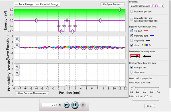Screenshot of Quantum Tunneling simulation You will use “Quantum Tunneling” PhET simulation to explore properties of matter wave, how it interacts with external potential, and how it responds when you make a measurement of particle position.

First, download the Java simulation and run it on your computer. Explore the simulation on your own for a while, until you feel comfortable with its features. Ask me any questions about different aspects of the simulation that you don’t feel that you understand. When you feel comfortable with the simulation (perhaps after 5 to 10 minutes), proceed with the instructions and questions below.

First, set up the simulation for the initial condition as following:

Choose Potential to be constant at 0 eV.
Choose Electron Wave Function view that you are comfortable with. If you have no preference, I recommend selecting “magnitude” and “phase” (but not “real part” or “imaginary part”).
After pausing the simulation, select the initial width and position of the wave. Select initial width of 1.0 nm, and choose the initial position as far to the left as possible that allows you to see the whole wave packet.

You are going to measure the uncertainty in the momentum of the wave packet, and this is how you will do it:

Note the initial position of the wave packet, and let the simulation run until the wave packet has almost reached the right edge of the screen. Pause the simulation.
Measure the distance that the peak of wave packet has traveled. Use the time measurement of the simulation to estimate the average speed and average momentum of the wave packet.
You should have seen the wave packet spreading noticeably. Use the spreading of the wave packet to estimate the uncertainty in momentum. That is, calculate a range of momenta contained within the initial wave packet.

Look up any physical constants needed. Please answer the questions below and follow further instructions.

Q1: What are the uncertainty in position ( $LaTeX: \Delta x = \sigma$ ) and momentum of the wave packet at the initial condition? Is this consistent with Heisenberg uncertainty principle? Explain your answer.

Q2: Make a measurement of the uncertainty in position when you paused the simulation (you will need to measure new width of the wave packet). Is this new value consistent with Heisenberg uncertainty principle? Explain your answer.

Q3: You can prepare a particle (i.e. wave packet) initial state in such a way that the initial uncertainty in position is small. However, the principles of wave mechanics says that, for a free particle, the uncertainty in position does not remain small. Explain conceptually why this is the case.

You can set up the simulation with a potential to reflect an incoming wave. Set up the simulation (after pausing it) as following for the next question:

Choose Potential to be “step.”
Set the energy values so that the energy before the step is -1.0 eV; the energy after the step is 0.5 eV, and the energy of the incoming particle is -0.5 eV.
Set the initial width of the particle to be 1.0 nm, with the initial position as far to the left of the screen as possible.

Run the simulation, you will see the wave packet bounce off from the step. Repeat the simulation as many times as necessary until you feel you have an understanding of what happened.

Q4: Does what you see agree with your intuition (which, mind you, is built up using Newtonian mechanics)? Explain how what you saw makes sense.

Lower the potential after the step to below -0.5 eV. Try running the simulation again and see what happens. (The sudden change in potential causes a portion of the wave to reflect off; it doesn’t really correspond to behavior of macroscopic objects, such as an airplane approaching and going over a cliff, but we can find classical waves, such as electromagnetic waves, that behave the same way.)

Now, set up the simulation with a barrier/well potential. We will observe a phenomenon called “quantum tunneling.” Set up the simulation as below:

Choose Potential to be “barrier/well”.
Set the energy values so that the energy before the barrier is -1.0 eV; the energy during the barrier is 0.5 eV; and the energy after the barrier is back to -1.0 eV. Leave the width of the barrier at the default value, you will be changing that in answering questions below.
Leave the particle state same as before.

Run the simulation, observing what happens with the wave packet. Repeat it as many times as necessary to understand what is going on.

Q5: Describe what happened with the wave packet. Does it agree with your intuition? Does it agree with your previous result?

During the interaction, you should have seen a significant portion of the particle wave packet enter into the barrier. So what you will do now is decrease the width of the barrier, so that the portion of the particle wave packet that enters into the barrier extends to the other side of the barrier. Run the simulation, observing what happens with the wave packet.

Q6: Describe what happens now. Explain what you would have expected to happen in classical mechanics (and why). Explain how what you see with wave mechanics is different (and why).

Q7: Find (“experimentally”) the width of the barrier that leads to 10% tunneling probability through the barrier. Give the width of the barrier in units of nanometers.

Reset the potential back to “constant,” and increase the particle energy back up to 0.5 eV. We are going to look at the effect of “quantum measurement.”

Q8: Pause the simulation, and click on “Make Quantum Measurement” (it makes measurement of particle position). Observe what happens to the wave function and the probability density. Does what you see make sense, based on what you know of electron (particle represented by the wave function), and what measurement does? Explain.

Q9: Unpause the simulation and observe what happens. Explain why what you observe happens.

One of the classical notion that we have to give up in quantum mechanics is the idea that you can make a measurement of a particle’s property (such as position and momentum) without affecting the state of the particle itself. In classical mechanics, it was an article of faith that you could make any disturbance due to a measurement as small as possible, so that the disturbance, in theory, was zero. In quantum mechanics, we admit to the fundamental limitation on how small we can make this disturbance due to a measurement, so the theoretical description of the particle state includes this fundamental uncertainty, and this leads to Heisenberg uncertainty principle. There are other formulations of quantum mechanics (“matrix mechanics”) that start out with this uncertainty principle as the founding assumption.

Part B: Fourier Analysis

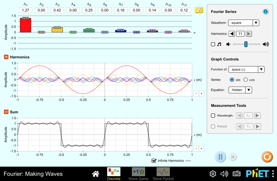Screenshot of Fourier simulation The position-momentum uncertainty principle can be understood as a natural consequence of position-wavelength uncertainty that already existed in classical mechanics (dealing with water waves, EM waves, sound waves, etc.). That is, once you accepted that a particle has wave property (through de Broglie hypothesis), then you should have expected this relationship between position and momentum uncertainty. The mathematical description of this position-wavelength uncertainty comes from Fourier analysis, and we will use the “Fourier: Making Waves” PhET simulation to help us explore some of the consequences (without actually having to do the integrals and other math involved in actual Fourier analysis).

“Fourier: Making Waves” is an HTML5 simulation and will run on all modern web browsers (mobile and on desktop). Explore the simulation on your own, until you feel comfortable with its features. As the simulation makes a lot of sounds, mute your computer audio except when you want to hear the sounds from the simulation. In “Discrete” tab, make sure to choose an equation form under “Equation” (default is “hidden”), under “Graph Controls.” This will display the mathematical expressions so that you can get into more detail, if you wish. Different representations are useful for different things. Explore!

Play with different “Waveform” functions, and observe how different waveforms, such as square waves and triangular waves are formed by combining sinusoidal waves of different harmonics. When you are ready, proceed to the question below.

Q10: In “Discrete” tab, choose “wave packet” as Waveform under Fourier Series. This will set up the harmonics so that you see a wave packet on the bottom graph. Toggle between “sin” and “cos” to see either odd or even wave packet. Describe how the wave packet is formed by superposition of all the harmonics selected. In particular, explain what is happening at the location where wave packet is at maximum amplitude (easier to visualize with cosines), and what is happening at the location where the wave packet sum is zero.

Q11: Under “Graph controls,” choose the wave to be a function of space and time. Observe what happens. Explain how it makes sense. (You can pause the simulation to stop the flow of time in the simulation, if you wish).

The wave packet you see above does not faithfully represent a single particle, mainly because the wave packet is periodic (you saw that in Q11). To obtain something that would represent a single particle, we have to go to the continuous limit. Switch to the “Wave Packet” tab.

Play with the simulation in this tab until you feel comfortable with different features here. Proceed when ready.

Set up the simulation for the initial condition by clicking the reset button on bottom right (looks like a refresh/recycle icon). Answer the questions below. Click the reset button between questions unless directed otherwise.

Q12: Describe what you see when you change the “Wave packet center.” The value of k₀ there represents the mean wavenumber (related to the average momentum by $LaTeX: p=\hbar k$ , in quantum mechanics). Observe how Amplitudes plot and Sum plot changes as you vary the wave packet center. Do the changes make sense?

Q13: Try changing the Wave packet width. The two sliders correspond to wave packet width in two different “spaces.” The first slider affects the wave packet width in the “k space” (also known as “momentum space” in quantum mechanics). The second slider affects the wave packet width in the “x space,” or “position space”. Describe what you see as you make the wave packet narrower either in k space or x space. Explain if the wave packet changes the way you expected. Also explain how wave packet width in k space is related to wave packet width in x space.

What you observed in Q13 is the fundamental reason behind the Heisenberg uncertainty principle (once you accept de Broglie hypothesis): you cannot make the wave packet narrower in position space without also making it wider in the momentum space. This connection is so intimate, that it works backward as well: there are formulations of quantum mechanics (to be covered in upper-division courses) where you start from Heisenberg uncertainty principle (as your fundamental, axiomatic assumption), and derive de Broglie relationship, rather than assuming it to start (“matrix mechanics”).

So far, you have dealt with periodic wave packets. Now we will see what is required (mathematically) to represent a single, spatially localized particle. First, zoom out on Sum graph as far as possible. Reduce the “Spacing between Fourier components.” Do it step by step (there are total of 3 steps), observing what happens with each step.

Q14: “Continuous limit” refers to when the spacing between Fourier components is zero. That is, the wave packet contains all the frequencies, within the envelope described by the wave packet width in k space. Describe what is required to mathematically represent a single particle localized within some space width width of $LaTeX: \sigma_x$ .

Q15: There exist particles known as “point particles” (one you know best is an electron). These are particles, as far as we know, do not have a finite size. As far as we can determine experimentally, these particles have no measurable size (i.e. no “radius of electron”), so we ought to be able to describe such point particle with a wave function of infinitesimally small width in position space. Describe some of the properties of such wave function. (For example, what frequency components does such a wave function contain?)

The “function” you described above is known as “Dirac delta function,” and you will learn more about it, if you take upper-division quantum mechanics.

Part C: Bound States

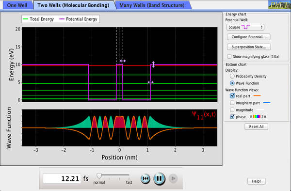Screenshot of Bound States simulation If you finished all the questions above and have some time left, you can explore the “Bound States” PhET simulation. This simulation simulates energy eigenstates in finite-well and Coulomb-type potentials. The double-well potential particularly is able to demonstrate the difference between states referred to as “stationary state” and “coherent superposition.”

If you have time to explore these, please call me and I will show you what settings to play with.